Gradient descent is the core mathematical mechanism that allows machine learning models to learn from empirical data. Every modern system that adapts, improves predictive accuracy, or trains on massive datasets depends fundamentally on some variation of this optimization strategy.
To understand how a machine learning model modifies its internal state, you must analyze how gradient descent in machine learning processes raw prediction errors and converts them into precise parameter updates that minimize overall model error.
This guide provides a comprehensive breakdown of the algorithm, tracing its mechanics from foundational mathematical principles through to the scaled implementation patterns used in production-grade artificial intelligence infrastructure.
What is Gradient Descent in Machine Learning?
At its most fundamental level, gradient descent is a first-order iterative optimization algorithm used to find the local minimum of a differentiable mathematical function. In the context of machine learning and deep learning, this function is almost always a loss function or objective function that quantifies the discrepancy between the predictions of a model and the actual ground-truth data points.
The primary objective during model training is straightforward: identify the exact configuration of model parameters, specifically the weights and biases, that minimizes this total prediction error.
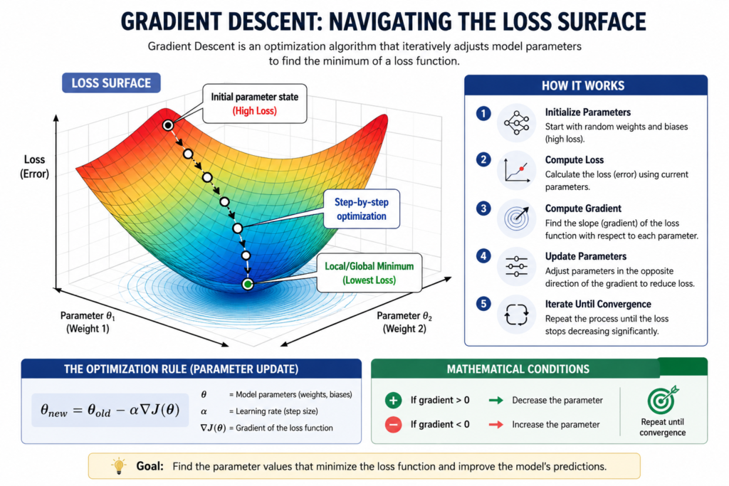
The algorithm functions by repeatedly adjusting these parameters in the exact direction that reduces the error value fastest, a path determined by calculating the local slope or gradient of the loss function surface.
Mathematically, the optimization logic operates under a strict set of conditions:
- If the calculated gradient is a positive value, the parameter value must be decreased.
- If the calculated gradient is a negative value, the parameter value must be increased.
- This cycle repeats systematically across multiple iterations until the system achieves convergence, the point where further updates yield no significant reduction in loss.
Why Gradient Descent is Central to Machine Learning Systems
Modern digital datasets routinely contain millions or billions of individual samples, and the models built to process them can feature hundreds of millions of parameters. Because of this massive scale, machine learning systems cannot use analytical math to solve for optimal parameters in a single step.
The mathematical surfaces of these loss functions are highly non-linear, complex, and high-dimensional. Calculating exact analytical solutions using classical matrix inversion techniques, such as solving the normal equation, becomes computationally impossible once a model incorporates thousands of intersecting features.
Instead of trying to find a perfect configuration immediately, machine learning infrastructure relies on efficient iterative optimization.
The gradient descent algorithm scales cleanly because it only requires computing local partial derivatives rather than calculating massive global matrices. This efficiency makes it the foundational training mechanic across a wide variety of models:
- Simple linear regression models predicting continuous values.
- Logistic regression classifiers mapping binary outcomes.
- Deep feedforward neural networks processing structural data arrays.
- Advanced transformer architectures managing complex language models.
Without this iterative framework, optimizing modern multi-layered neural network architectures would be completely impossible due to hardware memory bottlenecks and compute constraints.
How Machine Learning Uses Gradient Descent Step by Step
The operational execution of a gradient descent step can be broken down into a series of highly controlled data manipulation stages that occur within the training pipeline.
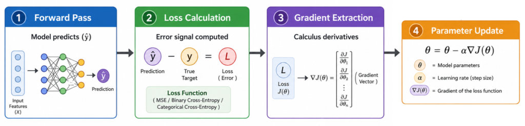
1. Model Makes Predictions
The optimization process begins with a forward pass where the model processes an incoming batch of features. The input features pass through the active network layers, multiplying against the current weights and adding the current biases to generate a definitive prediction output.
2. Loss Function Measures Error
The system evaluates the resulting prediction directly against the verified historical ground-truth target. The mathematical difference between these two values is processed through a targeted loss function, generating a clean numerical error signal.
The training framework switches its loss functions depending on the overall machine learning task:
- Mean Squared Error is standard for continuous regression tasks.
- Binary Cross-Entropy is utilized for two-class classification boundaries.
- Categorical Cross-Entropy is required for multi-class deep learning sorting.
3. Gradients Are Computed
Once the error signal is generated, the system extracts the learning signal by determining how much each individual weight and bias contributed to that specific error. This requires calculating the partial derivative of the loss function with respect to every separate parameter in the model.
This calculus step answers the core operational question: if a specific weight increases by a tiny fraction, will the total error go up or down, and by how much?
4. Parameters Are Updated Using Gradient Descent
With the directional gradients calculated, the system updates the internal parameters by shifting them in the direction that opposes the gradient vector.
The update process is governed by a precise mathematical equation:
θ=θ−α∇J(θ)
This update formula uses specific mathematical variables to control the training adjustment:
- θ represents the active model parameters being optimized.
- α represents the learning rate, a crucial hyperparameter that dictates the physical size of the adjustment step.
- ∇J(θ) represents the calculated gradient of the loss function across those specific parameters.
5. Iteration Across Epochs
This entire sequence is executed repeatedly across hundreds or thousands of training cycles known as epochs. The process continues until the model parameters stabilize, the loss curve flattens out completely, and the system reaches its optimized state.
Gradient Descent Algorithm (Core Training Logic)
The raw implementation of the training loop within modern machine learning frameworks follows a strict execution path that runs continuously until stopped by a human designer or an early stopping rule.
To implement this logic from scratch, an engineer configures a systematic program loop that processes data in this order:
- Initialize the model weights using random distribution values or specific normalization rules.
- Run the forward pass to compute the array of system predictions.
- Calculate the total scalar loss using the designated loss function.
- Execute the backpropagation step to pass the error backward and extract the parameter gradients.
- Apply the update formula to alter the internal weights.
- Repeat the entire sequence for a designated number of iterations or until the error change drops below a set threshold.
While this loop is mathematically simple, running it at a massive scale across parallelized hardware architectures is what powers nearly all modern artificial intelligence breakthroughs.
How Deep Learning Relies on Gradient Descent
In deep learning systems, the optimization landscape becomes significantly more complex than in classical linear models. Deep architectures feature thousands of intersecting hidden layers, highly non-linear activation functions, and parameter counts that can reach into hundreds of billions.
To update weights buried deep inside a neural network, the system uses an algorithm called backpropagation. Backpropagation works by utilizing the calculus chain rule to calculate the gradient of the loss function starting from the final output layer and passing it backward through each hidden layer.
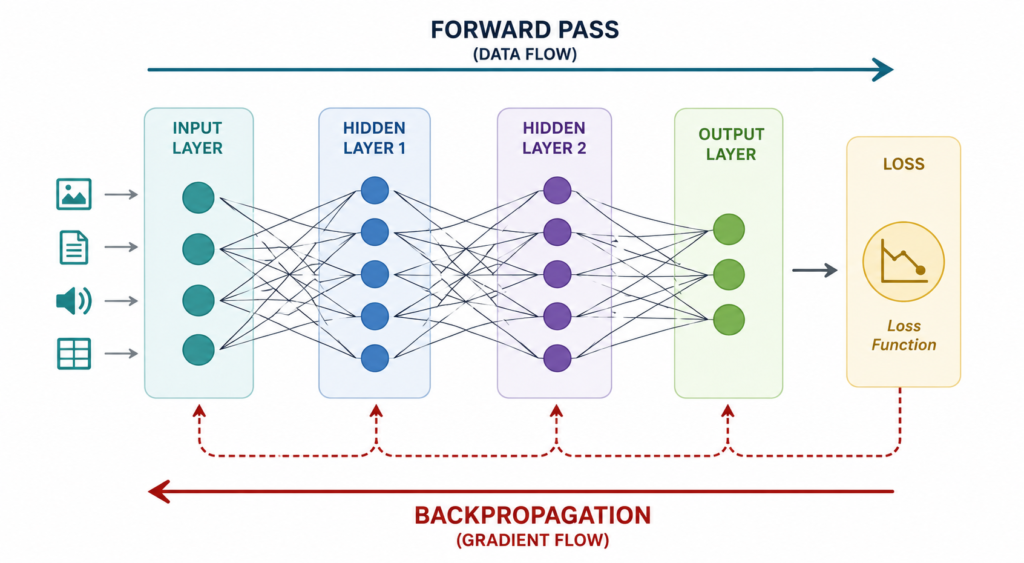
Without the structured application of gradient descent through backpropagation, multi-layer networks would fail to optimize their parameters:
- Convolutional Neural Networks would be unable to adjust their spatial filters to recognize edges, shapes, and complex visual objects.
- Transformer Models would fail to learn contextual relationships and linguistic associations across massive text tokens.
- Deep Autoencoders would fail to compress data or extract clean structural features from noisy input streams.
Gradient descent acts as the structural anchor that prevents deep networks from devolving into chaotic, un-trainable mathematical equations.
Variants of Gradient Descent Used in Real Systems
Standard gradient descent is rarely used in production-scale AI engineering because of memory limits and computational bottlenecks. Instead, engineers use specialized variants that balance computational efficiency with gradient precision.
The three core training frameworks include:
Batch Gradient Descent
This variation calculates the gradients for the entire dataset before applying a single parameter update. While it provides a stable learning trajectory, it requires massive amounts of hardware memory, making it incredibly slow and impractical for large modern datasets.
Stochastic Gradient Descent
This framework updates the model parameters immediately after processing each individual data sample. This approach is highly computationally efficient and runs fast, but the frequent updates cause the loss value to fluctuate wildly, resulting in an unstable training path.
Mini-Batch Gradient Descent
This approach splits the dataset into small, manageable chunks called mini-batches, typically ranging from 32 to 512 samples. It serves as the standard choice in production machine learning because it combines the stability of batch processing with the speed of individual sample updates.
Advanced Optimizers Built on Gradient Descent
To handle complex loss surfaces that contain flat plateaus, sharp valleys, and confusing directional changes, modern deep learning libraries rely on advanced optimization algorithms built on top of the core gradient descent formula.
Momentum
This technique tracks the velocity of past parameter updates to smooth out erratic training paths. By adding a fraction of the previous step to the current update, it helps the algorithm accelerate through flat surfaces and dampens unnecessary oscillations in narrow valleys.
RMSProp
This algorithm scales the learning rate dynamically for each individual parameter based on its recent gradient history. It divides the learning rate for a weight by a running average of the magnitudes of its recent gradients, which keeps updates stable when facing highly uneven surfaces.
Adam Optimizer
The Adaptive Moment Estimation optimizer combines the core principles of both Momentum and RMSProp. It tracks both the average velocity and the squared average of recent gradients, making it the highly reliable default optimizer for training deep neural networks and large language models.
Where Gradient Descent is Used in Real-World Systems
Gradient descent runs quietly behind the scenes of almost every major consumer and enterprise artificial intelligence application today.
The algorithm directly powers critical real-world systems across different industries:
- Digital Search Engines: Adjusting deep neural ranking models to optimize search relevance and deliver accurate content based on user intent.
- Streaming Recommendation Systems: Personalizing recommendations on platforms like Netflix and YouTube by continually updating collaborative filtering algorithms.
- Natural Language Processing: Training large transformer models to predict subsequent text tokens and handle nuanced conversational logic.
- Computer Vision Infrastructure: Powering real-time object detection systems, facial recognition programs, and diagnostic medical imaging tools.
- Financial Risk Core Systems: Optimizing predictive credit risk scoring models and processing live data inputs to detect credit card fraud.
Why Gradient Descent Works in High-Dimensional AI Models
Even when models contain billions of variables, gradient descent remains highly effective because high-dimensional spaces possess distinct geometric properties that actually aid optimization.
While early machine learning theories feared that models would get trapped in local valleys, data science research shows that high-dimensional loss surfaces are primarily populated by saddle points rather than true local minima. A saddle point is sloped upward in some directions but downward in others, allowing advanced optimizers with momentum to easily find an escape path and continue reducing overall error.
However, engineers must still monitor and mitigate three persistent hardware and training challenges:
- Vanishing Gradients: When gradients shrink exponentially as they travel backward through deep layers, causing early layers to stop learning entirely.
- Exploding Gradients: When gradients grow excessively large during backpropagation, causing the model weights to fluctuate wildly and destabilize training.
- Hyperparameter Sensitivity: Finding the right balance for the learning rate, as a value that is too high will cause the model to overshoot the minimum, while a value too low will make training incredibly slow.
Key Insight: Gradient Descent is the Core Learning Mechanism
Machine learning models do not understand data through human-like reasoning. Instead, learning is a process of continuous numerical optimization executed at an immense scale.
Every intelligent model is the direct historical byproduct of an iterative optimization loop that continuously measures error, calculates calculus gradients, and updates internal parameters. This simple, repetitive process serves as the underlying engineering engine that powers modern artificial intelligence systems.
Frequently Asked Questions
Why do AI models need gradient descent instead of exact formulas?
Modern models operate in high-dimensional spaces where calculating exact formulas requires massive matrix inversions that are computationally impossible for hardware to process. Gradient descent provides a scalable way to approximate the optimal configuration step by step.
How does gradient descent know if it is improving the model?
The algorithm monitors the output of the loss function. If the loss value decreases after an update, the model is successfully improving its predictive accuracy.
What happens if gradient descent is not properly tuned?
If the learning rate is set too high, the updates will overshoot the minimum and cause the training to fail. If it is set too low, the model will take too long to converge, driving up cloud computing costs.
Is gradient descent used in all types of machine learning models?
No. It requires a differentiable loss function, meaning it is used for neural networks, logistic regression, and linear regression. Non-differentiable models, like decision trees or random forests, use distinct split-efficiency calculations instead.
Why do deep learning models prefer mini-batch training instead of full datasets?
Mini-batch training balances computational efficiency with stable gradient directions, allowing engineers to maximize the parallel processing power of modern graphics processing units.
How does gradient descent scale to billions of parameters in modern AI systems?
It scales by splitting workloads across distributed clusters of specialized hardware like Graphics Processing Units and Tensor Processing Units, utilizing mini-batch tracking, and deploying efficient optimizers like Adam to keep updates stable.